Non-identifiability of LDS coordinates

An LDS's latent coordinates are identifiable only up to an invertible change of basis. For any invertible $S$, the transformed model $(A', Q', C', x_0', P_0') = (S A S^{-1},\, S Q S^\top,\, C S^{-1},\, S x_0,\, S P_0 S^\top)$ is observationally equivalent: same likelihood, same predictions. Here we demonstrate the equivalence numerically and show how Procrustes alignment lets us compare fits "apples-to-apples".

using StateSpaceDynamics
using LinearAlgebra
using Random
using Plots
using Statistics
using StableRNGs
using Printf

rng = StableRNG(1234);

Reference model

K_true = 3
D = 8
T = 200

A_true = [0.9  0.1  0.0;
         -0.1  0.8  0.2;
          0.0  0.0  0.7]
Q_true = 0.05 * Matrix(I(K_true))
b_true = zeros(K_true)

C_true = [1.0  0.5  0.0;
          0.8  0.3  0.1;
          0.2  1.0  0.0;
          0.0  0.7  0.4;
          0.1  0.2  0.9;
          0.3  0.0  0.8;
          0.6  0.4  0.2;
          0.4  0.6  0.5]
d_true = zeros(D)
R_true = 0.1 * Matrix(I(D))
x0_true = zeros(K_true)
P0_true = 0.2 * Matrix(I(K_true))

true_lds = LinearDynamicalSystem(;
    state_model=GaussianStateModel(A_true, Q_true, b_true, x0_true, P0_true),
    obs_model=GaussianObservationModel(C_true, R_true, d_true),
    latent_dim=K_true,
    obs_dim=D,
    fit_bool=fill(true, 6),
);

x_true, y_true = rand(rng, true_lds, T);

Equivalent transformed copies

A handful of similarity transforms: orthogonal rotations, an axis swap, a permutation, and a non-orthogonal scaling. All produce models with the same likelihood as the reference.

function transform_lds(lds, S)
    A_rot = S * lds.state_model.A * inv(S)
    Q_rot = S * lds.state_model.Q * S'
    C_rot = lds.obs_model.C * inv(S)
    x0_rot = S * lds.state_model.x0
    P0_rot = S * lds.state_model.P0 * S'
    return LinearDynamicalSystem(;
        state_model=GaussianStateModel(A_rot, Q_rot, b_true, x0_rot, P0_rot),
        obs_model=GaussianObservationModel(C_rot, lds.obs_model.R, d_true),
        latent_dim=size(A_rot, 1),
        obs_dim=size(C_rot, 1),
        fit_bool=fill(true, 6),
    )
end

transforms = [
    [cos(π/4) -sin(π/4) 0.0;  sin(π/4) cos(π/4) 0.0;  0.0 0.0 1.0],
    [1.0 0.0 0.0; 0.0 cos(π/2) -sin(π/2); 0.0 sin(π/2) cos(π/2)],
    Matrix(qr(randn(rng, K_true, K_true)).Q),
    [0.0 0.0 1.0; 0.0 1.0 0.0; 1.0 0.0 0.0],
    Matrix(Diagonal([2.0, 0.5, -1.2])),
    [0.0 1.0 0.0; 1.0 0.0 0.0; 0.0 0.0 1.0],
]
transform_names = [
    "rot(1,2, 45°)", "rot(2,3, 90°)", "random orthogonal",
    "axis swap (1↔3)", "scaling + sign", "permutation (1↔2)",
]

transformed_models = [transform_lds(true_lds, S) for S in transforms]

6-element Vector{LinearDynamicalSystem{Float64, GaussianStateModel{Float64, Matrix{Float64}, Vector{Float64}}, GaussianObservationModel{Float64, Matrix{Float64}, Vector{Float64}}}}:
 Linear Dynamical System:
------------------------
 Gaussian State Model:
 ---------------------
  State Parameters:
   A  = [0.85 0.15 -0.141; -0.05 0.85 0.141; 0.0 0.0 0.7]
   Q  = [0.05 0.0 0.0; 0.0 0.05 0.0; 0.0 0.0 0.05]
  Initial State:
   b  = [0.0, 0.0, 0.0]
   x0 = [0.0, 0.0, 0.0]
   P0 = [0.2 0.0 0.0; 0.0 0.2 0.0; 0.0 0.0 0.2]
  Dynamics input:
   size(B)  = (3, 0)
 Gaussian Observation Model:
 ---------------------------
  size(C) = (8, 3)
  size(R) = (8, 8)
  size(d) = (8,)
  size(D) = (8, 0)
 Parameters to update:
 ---------------------
  x0, P0, A (and b, B), Q, C (and d, D), R

 Linear Dynamical System:
------------------------
 Gaussian State Model:
 ---------------------
  State Parameters:
   A  = [0.9 6.12e-18 0.1; -6.12e-18 0.7 6.12e-18; -0.1 -0.2 0.8]
   Q  = [0.05 0.0 0.0; 0.0 0.05 0.0; 0.0 0.0 0.05]
  Initial State:
   b  = [0.0, 0.0, 0.0]
   x0 = [0.0, 0.0, 0.0]
   P0 = [0.2 0.0 0.0; 0.0 0.2 0.0; 0.0 0.0 0.2]
  Dynamics input:
   size(B)  = (3, 0)
 Gaussian Observation Model:
 ---------------------------
  size(C) = (8, 3)
  size(R) = (8, 8)
  size(d) = (8,)
  size(D) = (8, 0)
 Parameters to update:
 ---------------------
  x0, P0, A (and b, B), Q, C (and d, D), R

 Linear Dynamical System:
------------------------
 Gaussian State Model:
 ---------------------
  State Parameters:
   A  = [0.815 -0.0331 -0.0561; -0.106 0.791 0.179; 0.176 0.0346 0.794]
   Q  = [0.05 -1.39e-17 -1.73e-18; -1.39e-17 0.05 3.12e-17; 0.0 3.47e-17 0.05]
  Initial State:
   b  = [0.0, 0.0, 0.0]
   x0 = [0.0, 0.0, 0.0]
   P0 = [0.2 -5.55e-17 -6.94e-18; -5.55e-17 0.2 1.25e-16; 0.0 1.39e-16 0.2]
  Dynamics input:
   size(B)  = (3, 0)
 Gaussian Observation Model:
 ---------------------------
  size(C) = (8, 3)
  size(R) = (8, 8)
  size(d) = (8,)
  size(D) = (8, 0)
 Parameters to update:
 ---------------------
  x0, P0, A (and b, B), Q, C (and d, D), R

 Linear Dynamical System:
------------------------
 Gaussian State Model:
 ---------------------
  State Parameters:
   A  = [0.7 0.0 0.0; 0.2 0.8 -0.1; 0.0 0.1 0.9]
   Q  = [0.05 0.0 0.0; 0.0 0.05 0.0; 0.0 0.0 0.05]
  Initial State:
   b  = [0.0, 0.0, 0.0]
   x0 = [0.0, 0.0, 0.0]
   P0 = [0.2 0.0 0.0; 0.0 0.2 0.0; 0.0 0.0 0.2]
  Dynamics input:
   size(B)  = (3, 0)
 Gaussian Observation Model:
 ---------------------------
  size(C) = (8, 3)
  size(R) = (8, 8)
  size(d) = (8,)
  size(D) = (8, 0)
 Parameters to update:
 ---------------------
  x0, P0, A (and b, B), Q, C (and d, D), R

 Linear Dynamical System:
------------------------
 Gaussian State Model:
 ---------------------
  State Parameters:
   A  = [0.9 0.4 0.0; -0.025 0.8 -0.0833; 0.0 0.0 0.7]
   Q  = [0.2 0.0 0.0; 0.0 0.0125 0.0; 0.0 0.0 0.072]
  Initial State:
   b  = [0.0, 0.0, 0.0]
   x0 = [0.0, 0.0, 0.0]
   P0 = [0.8 0.0 0.0; 0.0 0.05 0.0; 0.0 0.0 0.288]
  Dynamics input:
   size(B)  = (3, 0)
 Gaussian Observation Model:
 ---------------------------
  size(C) = (8, 3)
  size(R) = (8, 8)
  size(d) = (8,)
  size(D) = (8, 0)
 Parameters to update:
 ---------------------
  x0, P0, A (and b, B), Q, C (and d, D), R

 Linear Dynamical System:
------------------------
 Gaussian State Model:
 ---------------------
  State Parameters:
   A  = [0.8 -0.1 0.2; 0.1 0.9 0.0; 0.0 0.0 0.7]
   Q  = [0.05 0.0 0.0; 0.0 0.05 0.0; 0.0 0.0 0.05]
  Initial State:
   b  = [0.0, 0.0, 0.0]
   x0 = [0.0, 0.0, 0.0]
   P0 = [0.2 0.0 0.0; 0.0 0.2 0.0; 0.0 0.0 0.2]
  Dynamics input:
   size(B)  = (3, 0)
 Gaussian Observation Model:
 ---------------------------
  size(C) = (8, 3)
  size(R) = (8, 8)
  size(d) = (8,)
  size(D) = (8, 0)
 Parameters to update:
 ---------------------
  x0, P0, A (and b, B), Q, C (and d, D), R

The invariant under any invertible $S$ is the marginal log-likelihood $\log p(y)$ (the latents are integrated out, so the volume Jacobian cancels). loglikelihood computes it exactly for a Gaussian LDS by running the Kalman filter and summing the one-step-ahead predictive densities. Note that the joint log p(x, y) at the smoothed mean (see joint_loglikelihood) is gauge-invariant only for orthogonal $S$; the diagonal scaling in transforms would shift it by $T \log |\det S|$.

ll_orig = loglikelihood(true_lds, y_true)

@printf("reference log p(y): %.6f\n", ll_orig)
for (name, S, model) in zip(transform_names, transforms, transformed_models)
    ll = loglikelihood(model, y_true)
    @printf("%-22s  ΔLL = %.3e  cond(S) = %.2f\n",
        name, abs(ll - ll_orig), cond(S))
end

reference log p(y): -725.349854
rot(1,2, 45°)           ΔLL = 0.000e+00  cond(S) = 1.00
rot(2,3, 90°)           ΔLL = 0.000e+00  cond(S) = 1.00
random orthogonal       ΔLL = 0.000e+00  cond(S) = 1.00
axis swap (1↔3)         ΔLL = 0.000e+00  cond(S) = 1.00
scaling + sign          ΔLL = 0.000e+00  cond(S) = 4.00
permutation (1↔2)       ΔLL = 0.000e+00  cond(S) = 1.00

Procrustes alignment

To compare two equivalent fits visually we solve $\hat S = \arg\min_S \lVert S X_\text{rot} - X_\text{orig} \rVert_F$ over orthogonal $S$, via SVD of $X_\text{orig} X_\text{rot}^\top$.

function procrustes_rotation(X, Y)
    F = svd(Y * X')
    return F.U * F.Vt
end

S_idx = 3
m_rot = transformed_models[S_idx]
x_orig, _ = smooth(true_lds, y_true)
x_rot, _ = smooth(m_rot, y_true)
S_hat = procrustes_rotation(x_rot, x_orig)

state_align_relerr = norm(S_hat * x_rot - x_orig) / norm(x_orig)
A_aligned = S_hat * m_rot.state_model.A * S_hat'
C_aligned = m_rot.obs_model.C * S_hat'
ΔA = norm(A_true - A_aligned)
ΔC = norm(C_true - C_aligned)

@printf("Procrustes residual: %.3e\n", state_align_relerr)
@printf("After alignment: ‖ΔA‖ = %.3e, ‖ΔC‖ = %.3e\n", ΔA, ΔC)

lim_A = max(maximum(abs, A_true), maximum(abs, A_aligned))
lim_C = max(maximum(abs, C_true), maximum(abs, C_aligned))

p_align = plot(layout=(2, 2), size=(900, 700))
heatmap!(p_align, A_true; title="A (true)", subplot=1, color=:RdBu,
    clims=(-lim_A, lim_A), aspect_ratio=:equal)
heatmap!(p_align, A_aligned; title="A (aligned)", subplot=2, color=:RdBu,
    clims=(-lim_A, lim_A), aspect_ratio=:equal)
heatmap!(p_align, C_true; title="C (true)", subplot=3, color=:RdBu,
    clims=(-lim_C, lim_C), aspect_ratio=:equal)
heatmap!(p_align, C_aligned; title="C (aligned)", subplot=4, color=:RdBu,
    clims=(-lim_C, lim_C), aspect_ratio=:equal)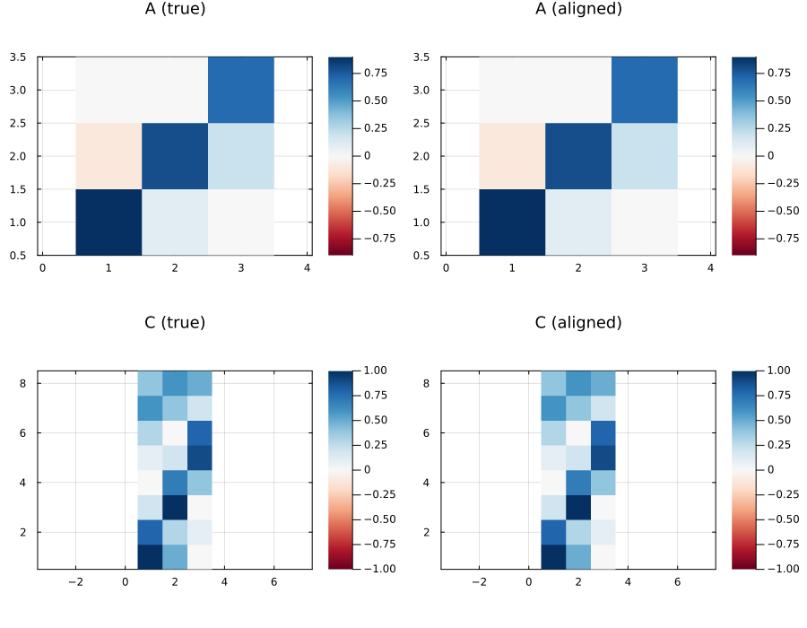

What is identifiable

Even though individual coordinates are gauge-dependent, three things are invariant under similarity transforms: eigenvalues of $A$ (and therefore modal timescales), the column space of $C$ (up to subspace angles), and all predictive metrics.

function subspace_angles_deg(C1, C2)
    Q1 = qr(C1).Q[:, axes(C1, 2)]
    Q2 = qr(C2).Q[:, axes(C2, 2)]
    σ = clamp.(svdvals(Q1' * Q2), -1.0, 1.0)
    return acos.(σ) .* (180 / π)
end

λ_true = sort(abs.(eigvals(true_lds.state_model.A)))
for (name, model) in zip(transform_names, transformed_models)
    λ = sort(abs.(eigvals(model.state_model.A)))
    θ = subspace_angles_deg(C_true, model.obs_model.C)
    @printf("%-22s  max|Δ|λ|| = %.2e  max angle(C) = %.3f°\n",
        name, maximum(abs.(λ_true - λ)), maximum(θ))
end

rot(1,2, 45°)           max|Δ|λ|| = 0.00e+00  max angle(C) = 0.000°
rot(2,3, 90°)           max|Δ|λ|| = 0.00e+00  max angle(C) = 0.000°
random orthogonal       max|Δ|λ|| = 2.22e-16  max angle(C) = 0.000°
axis swap (1↔3)         max|Δ|λ|| = 0.00e+00  max angle(C) = 0.000°
scaling + sign          max|Δ|λ|| = 0.00e+00  max angle(C) = 0.000°
permutation (1↔2)       max|Δ|λ|| = 0.00e+00  max angle(C) = 0.000°

This page was generated using Literate.jl.