Gaussian LDS
Here we simulate a 2-D rotational state-space system with Gaussian observations and recover the parameters with EM.
using StateSpaceDynamics
using LinearAlgebra
using Random
using Plots
using LaTeXStrings
using StableRNGs

rng = StableRNG(123);
Model
A Gaussian LDS evolves a latent state $x_t \in \mathbb{R}^D$ and emits an observation $y_t \in \mathbb{R}^p$ through
\[\begin{aligned} x_{t+1} &= A x_t + b + \varepsilon_t, & \varepsilon_t &\sim \mathcal{N}(0, Q), \\ y_t &= C x_t + d + \eta_t, & \eta_t &\sim \mathcal{N}(0, R). \end{aligned}\]
We pick $A$ as a contracting rotation so trajectories spiral inward.
obs_dim = 10
latent_dim = 2

A = 0.95 * [cos(0.25) -sin(0.25); sin(0.25) cos(0.25)]
Q = Matrix(0.1 * I(latent_dim))
b = zeros(latent_dim)
x0 = zeros(latent_dim)
P0 = Matrix(0.1 * I(latent_dim))

C = randn(rng, obs_dim, latent_dim)
R = Matrix(0.5 * I(obs_dim))
d = zeros(obs_dim);
Bundle the state and observation models into a LinearDynamicalSystem. fit_bool selects which parameter blocks are updated by EM. For a Gaussian LDS the six blocks are [x0, P0, A, Q, C, R], where the biases are folded into their regressions: b is fit jointly with A, and d jointly with C.
state_model = GaussianStateModel(; A=A, b=b, Q=Q, x0=x0, P0=P0)
obs_model = GaussianObservationModel(; C=C, d=d, R=R)
true_lds = LinearDynamicalSystem(;
    state_model=state_model,
    obs_model=obs_model,
    latent_dim=latent_dim,
    obs_dim=obs_dim,
    fit_bool=fill(true, 6),
);
Simulation
rand returns the latent trajectory and the observation matrix for a single trial of length tsteps.
tsteps = 500
latents, observations = rand(rng, true_lds, tsteps);
The latent dynamics form a smooth spiral; the observations are a noisy linear projection into a 10-dimensional space.
p_field = let
    x = y = -3:0.5:3
    X = repeat(x', length(y), 1)
    Y = repeat(y, 1, length(x))
    U = similar(X); V = similar(Y)
    for j in axes(X, 2), i in axes(X, 1)
        v = A * [X[i, j], Y[i, j]]
        U[i, j] = v[1] - X[i, j]
        V[i, j] = v[2] - Y[i, j]
    end
    mag = @. sqrt(U^2 + V^2)
    quiver(X, Y; quiver=(U ./ mag, V ./ mag), color="#898781", alpha=0.6)
    plot!(latents[1, :], latents[2, :];
        color=:black, linewidth=1.5, xlabel=L"x_1", ylabel=L"x_2",
        title="Latent dynamics", legend=false)
end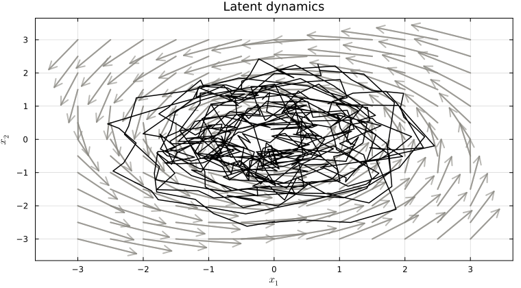
Latents on top, observations below.
p_traces = let
    lim_x = maximum(abs, latents)
    lim_y = maximum(abs, observations)
    p = plot(size=(800, 600), layout=@layout[a{0.3h}; b])
    for d in 1:latent_dim
        plot!(p, 1:tsteps, latents[d, :] .+ lim_x * (d - 1);
            color=:black, linewidth=2, label="", subplot=1)
    end
    plot!(p; subplot=1, title="Latents",
        yticks=(lim_x .* (0:latent_dim - 1), [L"x_%$d" for d in 1:latent_dim]),
        xticks=[], yformatter=y -> "")
    for n in 1:obs_dim
        plot!(p, 1:tsteps, observations[n, :] .- lim_y * (n - 1);
            color=:black, linewidth=1, label="", subplot=2)
    end
    plot!(p; subplot=2, title="Observations", xlabel="time",
        yticks=(-lim_y .* (obs_dim - 1:-1:0), [L"y_{%$n}" for n in 1:obs_dim]),
        yformatter=y -> "", left_margin=10 * Plots.mm)
end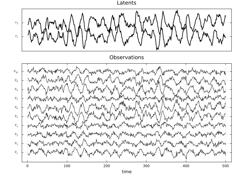
Smoothing
Given a (possibly wrong) parameter estimate, smooth returns the posterior mean and covariance of the latent state at each timestep. We start from a randomly initialised model so we can see how poor the estimate is before any learning.
naive_lds = LinearDynamicalSystem(;
    state_model=GaussianStateModel(;
        A=random_rotation_matrix(latent_dim, rng),
        Q=Matrix(0.1 * I(latent_dim)),
        b=zeros(latent_dim),
        x0=zeros(latent_dim),
        P0=Matrix(0.1 * I(latent_dim)),
    ),
    obs_model=GaussianObservationModel(;
        C=randn(rng, obs_dim, latent_dim),
        d=zeros(obs_dim),
        R=Matrix(0.5 * I(obs_dim)),
    ),
    latent_dim=latent_dim,
    obs_dim=obs_dim,
    fit_bool=fill(true, 6),
);

x_pre, _ = smooth(naive_lds, observations);
Learning
fit! runs EM until either max_iter or the relative-ELBO tol is hit, and returns the ELBO trajectory.
elbos = fit!(naive_lds, observations; max_iter=100, tol=1e-6);

x_post, _ = smooth(naive_lds, observations);
Fitting LDS via EM...   2%|█                                                 |  ETA: 0:01:06 ( 0.67  s/it)
Fitting LDS via EM... 100%|██████████████████████████████████████████████████| Time: 0:00:01 (16.57 ms/it)
The smoothed states track the true latents only up to an invertible change of basis (see the identifiability tutorial), so we undo the basis with the least-squares linear map before overlaying them. Applying the same alignment to the pre-EM estimate shows how much learning improves the recovery.
align_to_truth(x) = ((latents * x') / (x * x')) * x

x_pre_aligned = align_to_truth(x_pre)
x_aligned = align_to_truth(x_post);

p_compare = let
    lim_x = maximum(abs, latents)
    p = plot()
    for d in 1:latent_dim
        plot!(p, 1:tsteps, latents[d, :] .+ lim_x * (d - 1);
            color=:black, linewidth=2,
            label=(d == 1 ? "true" : ""), alpha=0.8)
        plot!(p, 1:tsteps, x_pre_aligned[d, :] .+ lim_x * (d - 1);
            color="#eda100", linewidth=1.5,
            label=(d == 1 ? "pre-EM (aligned)" : ""), alpha=0.6)
        plot!(p, 1:tsteps, x_aligned[d, :] .+ lim_x * (d - 1);
            color="#2a78d6", linewidth=2,
            label=(d == 1 ? "post-EM (aligned)" : ""), alpha=0.8)
    end
    plot!(p; title="True vs. recovered latents",
        yticks=(lim_x .* (0:latent_dim - 1), [L"x_%$d" for d in 1:latent_dim]),
        xlabel="time", yformatter=y -> "", legend=:topright)
end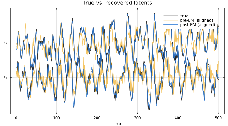
ELBO is guaranteed non-decreasing across EM iterations.
p_elbo = plot(elbos; xlabel="iteration", ylabel="ELBO",
    legend=false, linewidth=2, color="#2a78d6", title="EM convergence")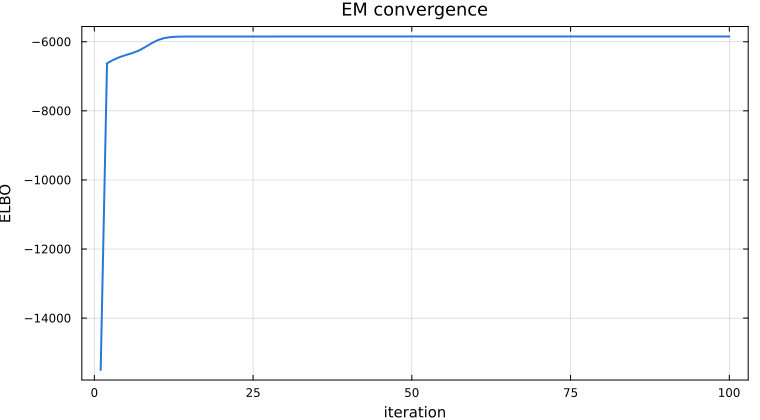
This page was generated using Literate.jl.